
MPPT and Output Voltage Regulation of a Photovoltaic System Based on Dual-stage Conversion and Nonlinear PI Control

Copyright© ICROS 2026
Abstract
The performance of solar photovoltaic systems is heavily dependent on environmental factors such as solar irradiance, ambient temperature, and partial shading. To maximize energy extraction under these variable conditions, maximum power point tracking (MPPT) algorithms are typically integrated with a boost converter; however, while MPPT ensures operation at the maximum power point, the resulting output voltage still fluctuates due to environmental and load variations. This study proposes a dual-stage conversion approach that simultaneously implements MPPT control and voltage regulation: the first stage employs a boost converter governed by the incremental conductance algorithm for maximizing power output, and the second uses a buck converter controlled by a nonlinear proportional-integral (NPI) controller to maintain a stable, desired output voltage. By integrating experimental data with a hybrid genetic algorithm, the photovoltaic cell parameters are identified and then applied to construct a detailed SIMULINK model for optimizing NPI controller gains. Finally, simulations are conducted to demonstrate the effectiveness of the proposed method, particularly under partial shading conditions.
Keywords:
photovoltaic, dual-stage conversion, maximum power point tracking, output voltage regulation, nonlinear PI control, hybrid genetic algorithmI. INTRODUCTION
Photovoltaic (PV) systems have emerged as a cornerstone in the global transition toward sustainable energy, driven by their global availability and the ability to convert sunlight directly into electricity efficiently [1]. As the demand for renewable energy sources escalates, PV technology has found diverse applications ranging from residential rooftops to large-scale solar farms, significantly contributing to energy independence and environmental preservation [2].
A vital step in getting the most out of PV systems is modeling and parameter estimation, especially when integrating maximum power point tracking (MPPT) and voltage regulation. These methods offer a mathematical framework that explains the system's behavior, allowing for optimized energy harvesting. This is done by identifying the ideal operating conditions, even in difficult situations like partial shading (PS). PS occurs when obstacles like trees, buildings, or dirt accumulation block sunlight from reaching the solar panels, leading to significant energy losses [3, 4]. The performance of PV systems can be hindered by environmental factors such as irradiance levels and temperature, with PS being particularly detrimental. To counteract these effects, various MPPT techniques have been developed to optimize energy extraction from PV modules [3-7]. Two of the most widely used methods are perturb and observe (P&O) and incremental conductance (InCon). Both are online algorithms, meaning they continuously find the maximum power point (MPP) by taking real-time measurements of the PV system's voltage and current [5]. However, they can struggle in dynamic environments, particularly when frequent shading changes occur. These changes introduce multiple local peaks in the power-voltage (P-V) curve.
In order to overcome the challenges of dynamic environments and PS, which cause multiple peaks in the P-V curve, several MPPT algorithms have been developed, each offering unique advantages and disadvantages. The modified adaptive hill climbing algorithm is accurate and adaptable, but computationally intensive and may respond slowly [6]. The constant voltage algorithm is simple and maintains a steady voltage near the maximum power point, but lacks adaptability [7]. The lookup table-based algorithm uses precomputed data for quick adjustments, relying on the quality of the lookup table [8]. Model predictive control predicts optimal operating points using system models and has been applied in ultra-step-up boost converters [9]. Metaheuristic optimization, such as particle swarm optimization and genetic algorithms treat the MPPT problem as an optimization challenge, systematically searching the entire P-V curve to find the absolute MPP [10,11]. However, a key disadvantage of these approaches is the difficulty in evaluating the performance of all potential individuals in the population within a practical, finite time when implemented in an actual PV system. More critically, the presence of even a few bad individuals can drastically lower the overall performance of the system.
The challenge in PV systems arises because even though the MPPT stage constantly adjusts the system to maintain the PV array at its MPP, the resultant output voltage is inherently variable and unstable due to changing environmental conditions. This variable voltage is generally unsuitable for the downstream load or grid, which critically requires a highly stable, fixed DC voltage for proper operation. Therefore, the separate voltage-regulation stage is essential for decoupling the power optimization task from the voltage stabilization task, ensuring that the maximum power extracted by the MPPT stage is delivered with the necessary quality and stability for utilization by external systems. While traditional control strategies, such as proportional-integral-derivative (PID) controllers, have been used to maintain output voltage, they often fail to adequately address the complexities introduced by PS [12]. Recent advancements in intelligent control methods, such as fuzzy logic and neural networks [13], show promise but often require extensive tuning and adaptation to specific system configurations. While various MPPT and voltage regulation techniques exist, as indicated above, most studies focus separately on either MPPT or voltage regulation in PV systems rather than addressing both simultaneously [14].
This study presents an integrated control approach that optimally combines MPPT and output-voltage regulation via a dual-stage power-conversion system. In the MPPT stage, a boost converter is employed, and its operation is controlled by the InCon algorithm to achieve effective MPPT. Following this, in the voltage regulation stage, a buck converter is utilized, and its output voltage is stably maintained using a nonlinear proportional-integral (NPI) controller. To achieve the research goals, the work will begin by selecting an appropriate PV cell model and determining its parameters using experimental data. This crucial parameter estimation will be performed with a hybrid genetic algorithm (HGA) [15], which is essential for accurate system modeling, effective implementation of the control strategy, and the subsequent optimization of the NPI controller's gains. Finally, the performance of the two integrated control methods will be assessed through a series of MATLAB SIMULINK simulations. These simulations will be evaluated across four different irradiance scenarios to thoroughly enhance PV system efficiency and ensure stable operation under variable environmental conditions, including PS.
II. IDENTIFICATION OF A PV CELL
Successful design and analysis of a PV system begins with identifying the controlled object, which requires prior knowledge of the PV cell model. The PV cell identification task is broken down into four key steps: data collection, model selection, parameter estimation, and model validation. The resulting model will then be applied to the MPPT control and controller design for voltage regulation in the subsequent section.
1. Model Selection of a PV Cell
A solar cell can be modeled using various approaches, including single-diode and two-diode models [16]. This work utilizes the single-diode model, represented by an electrical equivalent circuit composing a constant current source in parallel with a diode, as illustrated in Fig. 1.
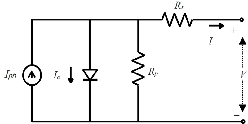
Equivalent circuit of a PV cell.
To obtain a model from the equivalent circuit and estimate its parameters, data are obtained from a reference module under standard test conditions (STC), which are a cell temperature of 25℃, a solar irradiance of 1,000W/m², and an air mass of 1.5. Under STC, the output current I can be expressed by [12]
| (1) |
where V and I are the output voltage and current of a PV cell, respectively; Iphr, Ior, Rs, Rp, a and Tr are the photodiode current, the reverse saturation current, the series resistance, the shunt resistance, the ideality factor, and the reference temperature at STC, respectively; K is the Boltzmann constant (= 1.38×10⁻²³ J/K) and q is the charge of an electron (= 1.6×10⁻¹⁹C).
However, varying solar irradiance and temperature in a real environment may change these parameters. In this case, Equation (1) can be rewritten by
| (2) |
where Iph, Io and T are the photodiode current, the reverse saturation current, and the temperature in a real environment, respectively. The relationship between the parameters in Equations (1) and (2) is as follows:
| (3) |
| (4) |
where Ki denotes the short-circuit current temperature coefficient, G the solar irradiance (W/m²), Gr the nominal solar irradiance (typically 1,000W/m²), and Eg the bandgap energy of the semiconductor.
A single PV cell typically generates a low power output between 1 to 2 watts under STC. To amplify the overall output, multiple PV cells are connected in series and/or parallel, encapsulated within a protective frame and materials, known as a PV module. The model of a PV module composed of Np parallel cells and Ns series cells is defined by
| (5) |
where V and I mean the output voltage and current of the PV module, respectively; Λ = Ns / Np ; RsΛ and RpΛ denote the equivalent series and parallel resistances of the PV module, respectively.
2. Parameter Estimation of the PV Module
The next phase is to estimate the five unknown parameters (Iph, Io, a, Rs and Rp) of the PV module. This is done using voltage ( V ) and current ( I ) measurements. The Kyocera KC200GT module is selected as the reference. Under STC, this module with Ns =54 and Np =1 exhibits voltage ranging from 0 to 32.9V and current ranging from – 2.65 to 8.23A. At STC, Iph and Io are equal to their reference values, Iphr and Ior, respectively. These are estimated from the measured data set of {V, I} using n optimization technique. By rearranging the terms, Equation (4) becomes
| (6) |
where x = [Iph, Io, a, Rs, Rp]T · f(x,V,I) represents the error between the physical PV module and the model. The objective of parameter estimation is to tune the five parameters to minimize the performance index. To quantitatively evaluate the goodness-of-fit for different parameter sets, the root mean square error (RMSE) is used as the performance index.
| (7) |
where M denotes the total number of collected I – V data points; in this study, M = 69.
Ultimately, estimating the five parameters results in a multivariate optimization problem. The HGA is used to solve this problem by minimizing Equation (7) within a defined search space: X = {x | x(L) ≤ x ≤ x(U) }, where x(L) and x(U) represent the lower and upper bounds of x , respectively. The procedure of the HGA is as follows [15]:
- Step 1: Initialize a population of size N randomly;
- Step 2: Evaluate individuals via Equation (7) and determine the global best xglobal(t) and its function value fglobal(t), and the local worst function value fworst(t);
- while <Termination criterion is not met> do Steps 3-5
- Step 3: Perform the affine combination-based reproduction to update each individual xi(t) as
| (8) |
| (9) |
-
- where xi(t) and fi(t) are an individual and its function value, respectively. ηi is a positive constant defined by the user and is drawn from a Gaussian distribution N(η, σ2), where η is the mean and σ is the standard deviation. As a result, each individual receives a value typically close to η, subject to some degree of variation.
- Step 4: Perform the non-uniform mutation [17]:
| (10) |
| (11) |
-
- where xj is the chosen gene, is the mutated gene, τ is a random digit (0 or 1), r is a uniform random number, tmax is the maximum number of generations and b is the shape parameter.
- Step 5: Evaluate individuals via Equation (7) and determine xglobal(t), fglobal(t), and fworst(t);
- end while
For the HGA, the parameters are configured as follows: a population size of N=40; reproduction settings with η= 1.8 and σ= 0.01; non-uniform mutation probability Pm =0.04 and b=6. The search bounds were defined by the lower bound x(L) = [0,0,0,0,0]T and the upper bound x(U) = [20,0.1,5,1,400]T. These ranges were established via preliminary simulations to guarantee comprehensive exploration of the parameter space. The maximum number of generations was set to 4000. The HGA's convergence capability and speed are highly sensitive to the randomly generated initial population. Therefore, to obtain reliable, stable results, we conducted 20 independent runs with different random seeds. Subsequently, Table 1 averaged the resulting estimated parameters.

Parameter estimates of the single diode model.
3. Model Validation
To validate the estimated model, the I-V and P-V characteristics curves were plotted against the measured data in Fig. 2. The agreement was statistically confirmed by an R-squared (R2) value of 99.98 %, indicating excellent agreement between the HGA-based estimated parameters and the measured data. Further analysis of the estimated model's performance begins with Fig. 3, which displays the I-V and P-V curves under varying temperatures at a constant irradiance of 1,000W/m2. Following this, Fig. 4 shows the I-V and P-V curves under varying irradiance levels at a constant temperature of 25°C.
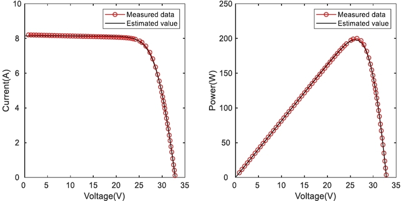
I-V and P-V characteristics of measured data and the estimated model at STC.
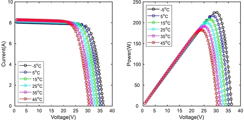
I-V and P-V characteristics of the estimated model under varying temperature at an irradiance of 1,000W/m2.
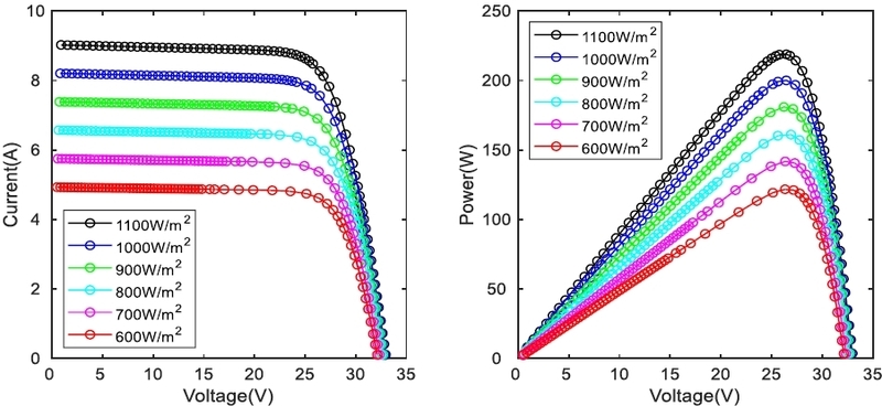
I-V and P-V characteristics of the estimated model under varying irradiance at a temperature of 25℃.
III. CONTROL STRATEGY FOR THE PV SYSTEM
1. Proposed Control Strategy
The proposed PV control strategy utilizes a dual-stage conversion system, implementing a decoupled control scheme in Fig. 5. In this scheme, the first-stage (boost converter) handles MPPT, while the second-stage (buck converter) manages output voltage regulation. This separation of control tasks is crucial for ensuring maximum energy extraction while maintaining a stable power output.
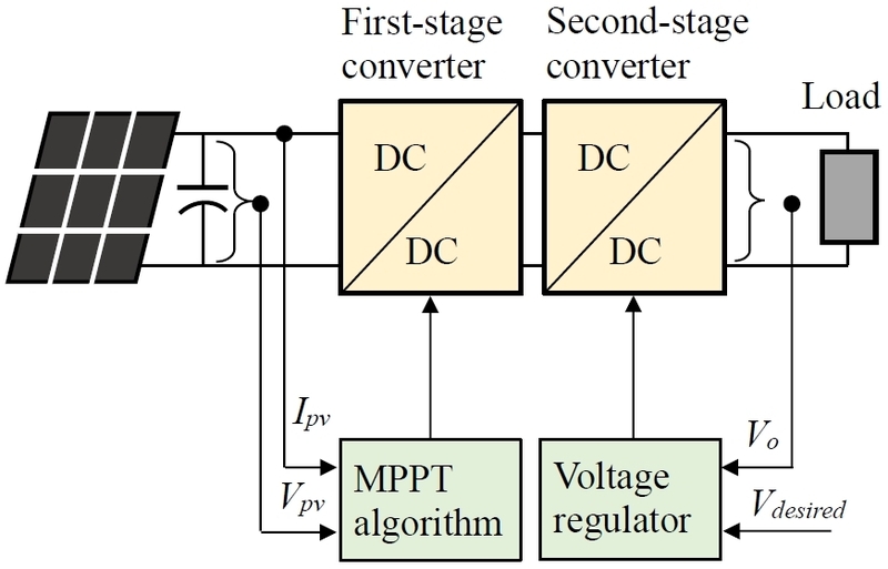
Block diagram of the dual-stage conversion system for the PV system.
2. MPPT Algorithm
The first-stage converter, directly connected to the PV panel, is controlled by an MPPT algorithm to produce the maximum power output under a given set of environmental conditions. The boost converter's duty cycle is continuously regulated by the MPPT algorithm.
A number of MPPT algorithms have been proposed in the literature, including P&O and InCon [18]. We utilize the popular and high-performing InCon algorithm, which is briefly summarized here.
The InCon algorithm operates based on the fundamental relationship between the instantaneous slope of the P-V curve and the MPP. The slope of the P-V curve is obtained by taking the derivative of the power (P = V · I) with respect to voltage (V ):
| (12) |
where dI / dV represents the incremental conductance, and I / V represents the instantaneous conductance. The algorithm constantly compares the two values from Equation (12) to guide the operating point toward the MPP. This slope is then used to determine the direction in which the operating voltage must be changed:
- • At MPP = 0, then = −
- • Left MPP > 0, then > − (Increase V to move right towards MPP)
- • Right MPP < 0, then < − (Decrease V to move left towards MPP)
3. Nonlinear PI Controller
The first-stage boost converter produces a variable voltage because it tracks the MPP under changing environmental conditions. The subsequent buck converter must stabilize the fluctuating input to maintain a constant output voltage (Vo) for the load. This can be managed by a feedback control loop (typically PID), which measures Vo, compares it to the desired setpoint (Vdesired), and adjusts the buck converter's duty cycle to maintain the required constant output output.
However, due to the high-frequency switching ripple from PWM operation in the converters, the derivative term in standard PID controllers is problematic, as it amplifies this ripple, leading to instability and chattering. Consequently, the derivative term is often filtered or omitted. We therefore employ a NPI controller, a modification of the author's nonlinear PID controller [19]. The NPI controller is of the following form:
| (13) |
| (14) |
where u and u0 are the control input and the nominal control input, respectively, e is the error between the setpoint and the output voltage, and Kp and Ki are the proportional and integral gains, respectively. v(t) is the scaled error and k(e) is a nonlinear gain defined as:
| (15) |
where b is a positive constant and σ is a user-defined constant. Substituting (15) in (13) gives
| (16) |
To ensure the nonlinear gain amplifies small errors for offset reduction while attenuating larger errors to prevent accumulation, b is selected so that v(t) matches e(t) specifically when e(t) reaches the threshold σ.
| (17) |
By rearranging (17) and substituting the result into (15), the following equation is obtained:
| (18) |
Fig. 6 shows the error plots before and after scaling with a typical value of σ =1.
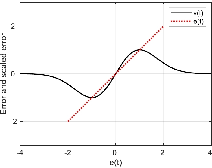
Error plots before and after scaling.
The NPI controller's integral action can improve control performance by slightly increasing small errors to accelerate convergence and by scaling down large errors to prevent the cumulative error from growing excessively. This scaling is crucial because the unrestricted accumulation of error, known as integral windup, leads to significant performance degradation, causing large overshoots, delayed recovery, increased oscillation, and instability. Setting σ to one-third of the maximum setpoint change is recommended for a desirable response.
4. Optimum Tuning of the NPI Controller Using the HGA
Like other controllers, the NPI controller relies on its two gains (Kp, Ki) for effective voltage regulation. Traditional empirical tuning methods are unsuitable due to the NPI's nonlinear element. Consequently, we use another HGA to optimize the gains based on the MATLAB/SIMULINK model. The optimization utilizes the integral of absolute error (IAE) as the performance measure.
| (19) |
where e(t) is the difference between the setpoint and the output voltage as e(t)=Vdesired(t)-Vo(t).
IV. SIMULATION AND RESULT DISCUSSION
The proposed method was validated through simulations performed in SIMULINK, utilizing the model illustrated in Fig. 7. The overall system comprises serially connected PV modules (Kyocera KC200GT), the boost and buck converters, the InCon algorithm, the NPI controller, and a load.
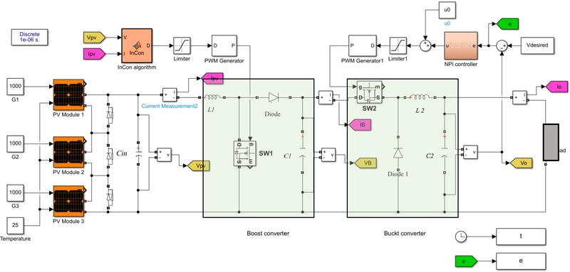
SIMULINK model for implementing the dual-stage DC-DC converter system.
1. Design of the Two Converters
The SIMULINK model for the dual-stage DC-DC converter was built by defining specific component parameters. The input source uses three series-connected PV panels rated for a maximum power of 600W (VMPP = 26.3V, IMPP = 7.61A at STC). The boost and buck converters are designed for output voltages of 100V and 32V, respectively. Utilizing a conservative 90% system efficiency and setting ripple constraints (max output voltage ripple ≤ 1%; max input current ripple ≤ 30%; input PV voltage ripple ≤ 0.5%), the component parameter values are provided in Table 2. The calculated minimum input necessary capacitance (Cin) to meet the voltage ripple constraint is 7.22μF.
Designed component values.
2. Controller Gain Settings
The gains of the NPI controller were optimized using the SIMULINK model (Fig. 7), under STC. The optimization employed the HGA using the same parameters as described in Section II and the two gains were searched within the bound 0<Kp, Ki<3. For a fair comparison, the NPI controller's performance was benchmarked against the standard PI controller. The PI controller gains were also optimized by minimizing the performance index defined in Equation (19). The final optimized results for both the NPI and PI controllers are presented in Table 3.
Optimized gains of the NPI and PI controllers.
3. Performance Test
The designed system was simulated under two distinct conditions: STC and PS. PS was modeled to account for typical causes like shadows and varying solar angles. Temperature variations were excluded from the study because they change much more slowly than irradiance. Consequently, the temperature was kept constant at 25°C. The responses and comparative performance of the two control methods were evaluated across four distinct irradiance scenarios. For quantitative analysis, the following metrics were calculated: overshoot (Mp), rise time (tr), settling time (ts) and IAE as defined in (19).
To simplify nomenclature for the comparison, the system combining the NPI controller and the InCon algorithm is denoted as NPI-InCon. Similarly, the combination of the PI controller and the InCon algorithm is referred to as PI-InCon.
All panels were assumed to operate under STC. The desired voltage was stepwisely changed from 0V to 32V. Fig. 8 displays the resultant buck converter's output voltage and power responses to this voltage change. As anticipated, the HGA-optimized gains ensured both the NPI and PI controllers achieved the required voltage within 0.4ms. The responses exhibit a minor initial oscillation, primarily due to the MPPT process using the InCon algorithm. The quantitative performance metrics are summarized in Table 4. Analysis of these values indicates that the PI-InCon method marginally outperformed the NPI-InCon method.
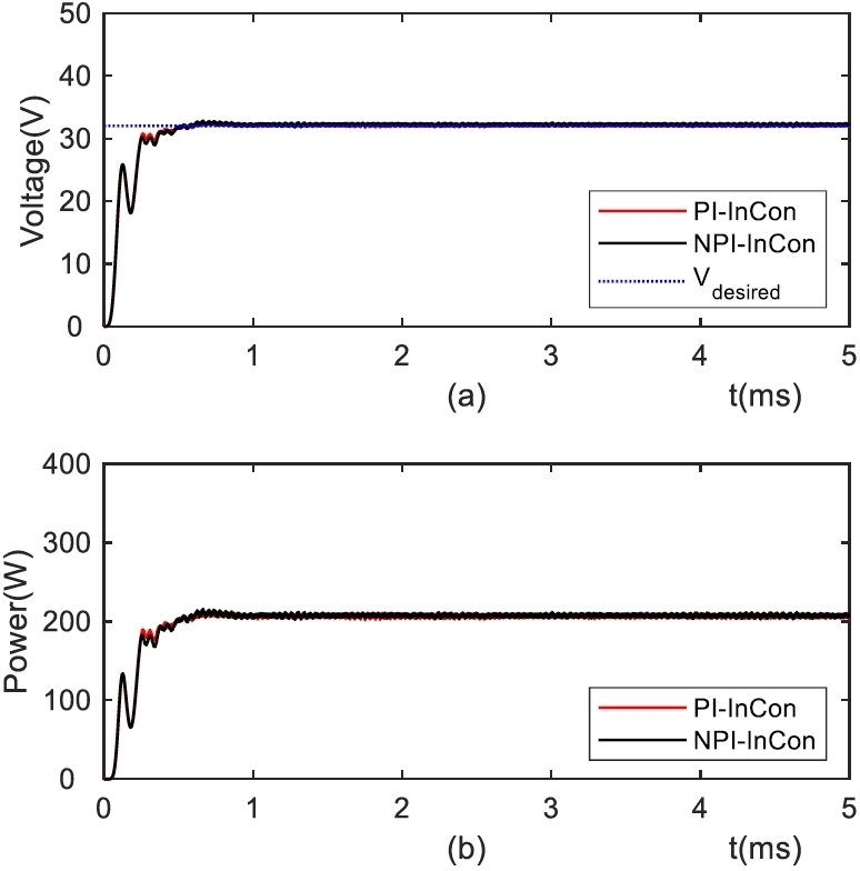
Output of the buck converter to stepwise setpoint change for Case 1: (a) voltage, (b) power.
Quantitative performance comparison of the two methods for Case 1.
The subsequent simulation was performed under constant PS conditions, where the three panels received unequal irradiance: G1 =1000W/m2, G2 =600W/m2, and G3 =400W/m2. Fig. 9 illustrates the controllers' responses to the same stepwise voltage input.
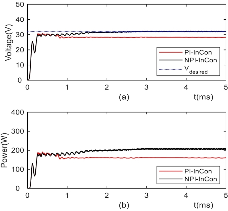
Output of the buck converter to stepwise setpoint change for Case 2: (a) voltage, (b) power.
Despite reduced power output due to shading, the NPI-InCon method reached the setpoint quickly, settling within approximately 1.3ms. In contrast, the PI-InCon method performed poorly, failing to settle even within 5ms. This observed failure of the PI-InCon method stems from the static nature of its gain tuning at STC, which proves inadequate when the setpoint shifts under PS conditions.
Table 5 summarizes the quantitative performance metrics. Based on these calculated values, the NPI-InCon method demonstrated superior effectiveness compared to the PI-InCon method under the tested conditions.
Performance comparison of the two methods for Case 2
This simulation was conducted under dynamic PS conditions. The three PV panels, initially operating at STC, were progressively shaded over time. The specific shading profile applied is as follows: At 30ms, G3 drops from 1000W/m2 to 400W/m2. At 60ms, G2 drops from 1000W/m2 to 600W/m2. This time-varying irradiance profile is shown graphically in Fig. 10(a). Figs 10(b) and 10(c) show the system responses to the same stepwise input, while Fig. 10(d) depicts the resulting changes in the duty cycle.
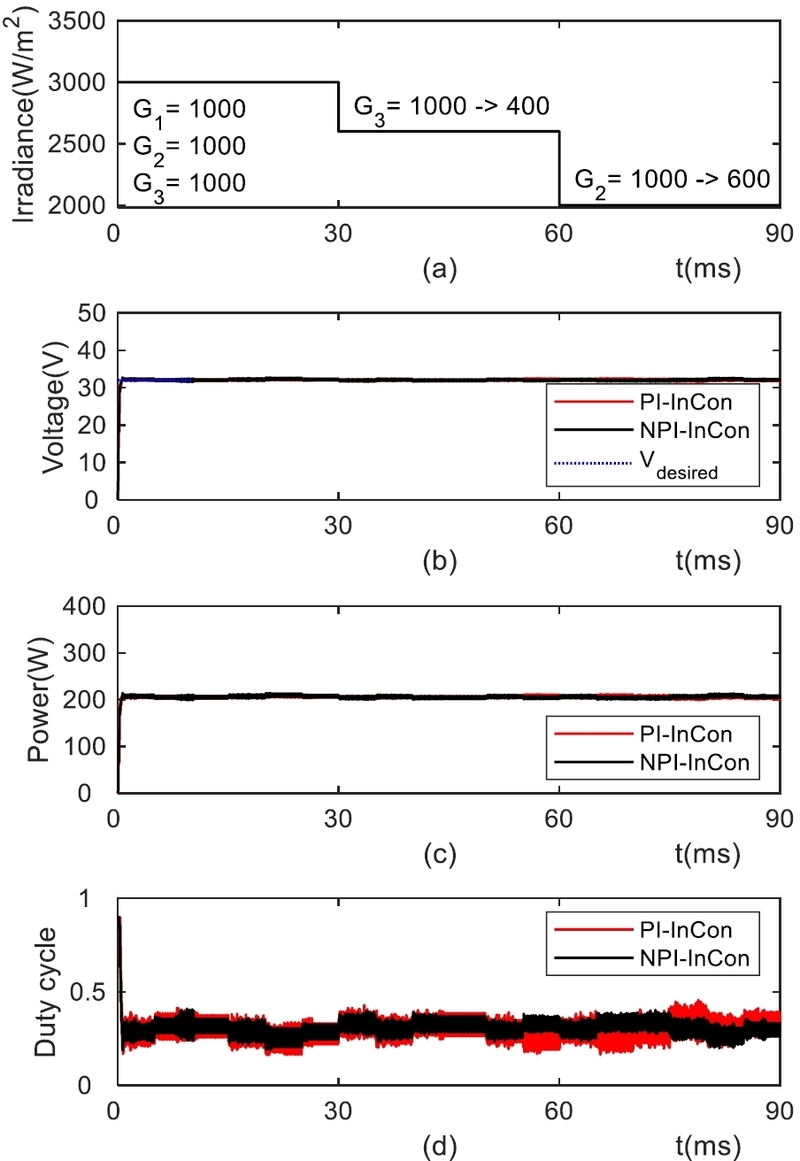
Output of the buck converter to stepwise setpoint change for Case 3: (a) irradiance, (b) voltage, (c) power, (d) duty cycle.
Both controllers maintained the output voltage consistently near the setpoint under shading conditions. For quantitative evaluation, their IAEs were calculated. Although the PI-InCon method showed a marginally smaller IAE of 19.03 compared to the NPI-InCon method's 19.93, the duty cycle response of the PI-InCon method displayed larger fluctuations than that of the NPI-InCon method.
The final simulation investigated the system's responses to dynamic irradiance restoration. The test began under an initial PS state, with irradiances set at G1 =1000 W/m2, G2 =600W/m2, and G3 =400W/m2. The shading was then progressively removed in two stages: At 30ms, G2 was restored from 600W/m2 back to 1000W/m2 (STC). At 60ms, G3 was restored from 400W/m2 to 1000W/m2.
Fig. 11 shows the system's response to dynamic irradiance restoration. Specifically, Fig. 11(a) illustrates the irradiance test profile, while Figs. 11(b) and 11(c) show the resulting output voltage and delivered power for both control methods. Finally, Fig. 11(d) depicts the corresponding switching duty cycle used to regulate the converter.
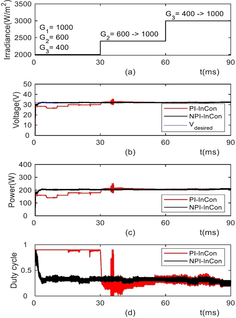
Output voltage and power of the buck converter to stepwise setpoint change for Case 4.
In Case 4, the output voltage behavior varied significantly between the two methods. The output voltage of the PI-InCon method reached the setpoint only after G2 was partially restored around 30ms. On the other hand, the NPI-InCon method maintained the output voltage at the setpoint consistently, regardless of the shading restoration event. For quantitative assessment, the IAEs were calculated. The NPI-InCon method demonstrated vastly superior performance with an IAE of 20.07, compared to the PI-InCon method's high IAE of 116.68. Regarding the duty cycle response, the NPI-InCon's duty cycle remained comparatively stable with smaller fluctuations, while the PI-InCon's duty cycle displayed significantly larger fluctuations, reflecting its poorer stability during the transient event.
V. CONCLUSION
This study introduced and evaluated a control strategy for a PV system utilizing a dual-stage conversion system, featuring a decoupled approach: InCon-based MPPT on the boost stage and voltage regulation on the buck stage. For the first task, the PV cell identification was carried out to estimate the parameters of a PV cell model. The core of this strategy is to use the effective NPI controller for output voltage regulation, whose gains were optimized using the HGA. A set of simulations were conducted using the SIMULINK model. The responses and performance of the two control methods were evaluated across four distinct irradiance scenarios.
Simulation results confirmed that both the NPI-InCon and PI-InCon methods provided rapid voltage regulation under STC, settling within 0.4ms. Crucially, the NPI-InCon demonstrated significant superiority under PS: in constant shading, NPI achieved the setpoint in approximately 1.3ms, substantially faster than the PI-InCon's stabilization time of over 5ms. Furthermore, in dynamic shading scenarios, the NPI-InCon method exhibited smaller steady-state duty-cycle fluctuations, indicating better dynamic stability. Overall, the NPI controller provides greater effectiveness in voltage regulation and power harvesting efficiency in PV systems than the conventional PI controller.
REFERENCES
-
S. Al-Ali, A. G. Olabi, and M. Mahmoud, “A review of solar photovoltaic technologies: developments, chal-lenges, and future perspectives,” Energy Conversion and Management: X, vol. 27, pp. 101057, Jul. 2025.
[https://doi.org/10.1016/J.ECMX.2025.101057]

-
M. A. Green, E. D. Dunlop, J. Hohl-Ebinger, M. Yoshita, N. Kopidakis, and X. Hao, “Solar cell efficiency tables (version 56),” Progress in Photovoltaics: Research and Applications, vol. 28, no. 7, pp. 629–638, Jul. 2020.
[https://doi.org/10.1002/pip.3303]
-
E. H. Sepúlveda-Oviedo, “A review of operational factors affecting photovoltaic system performance,” Energy Conversion and Management: X, vol. 26, pp. 100942, Apr. 2025.
[https://doi.org/10.1016/J.ECMX.2025.100942]
-
J. Bai, Y. Cao, Y. Hao, Z. Zhang, S. Liu, and F. Cao, “Characteristic output of PV systems under partial shading or mismatch conditions,” Solar Energy, vol. 112, pp. 41–54, Feb. 2015.
[https://doi.org/10.1016/j.solener.2014.09.048]
-
F. Belhachat and C. Larbes, “Comprehensive review on global maximum power point tracking techniques for PV systems subjected to partial shading conditions,” Solar Energy, vol. 183, pp. 476–500, May 2019.
[https://doi.org/10.1016/J.SOLENER.2019.03.045]
-
W. Xiao and W.G. Dunford “A modified adaptive hill climbing MPPT method for photovoltaic power systems,” In Proceedings of the PESC Record–IEEE Annual Power Electronics Specialists Conference, 3 (2004), pp. 1957-1963, 2004.
[https://doi.org/10.1109/PESC.2004.1355417]
-
K.A. Aganah and A.W. Leedy, “A constant voltage maximum power point tracking method for solar powered systems,” In Proceedings of the 2011 IEEE 43rd Southeastern Symposium on System Theory, Auburn, AL, USA, pp. 125–130, 14–16 March 2011.
[https://doi.org/10.1109/SSST.2011.5753790]
-
V.R. Kota and M.N. Bhukya, “A simple and efficient MPPT scheme for PV module using 2-dimensional lookup table,” Proceedings of the 2016 IEEE Power and Energy Conference at Illinois (PECI), Urbana, IL, USA, pp. 1–7, 19–20 February 2016.
[https://doi.org/10.1109/PECI.2016.7459226]
-
L. Samani and R. Mirzaei “Maximum power point tracking for photovoltaic systems under partial shading conditions via modified model predictive control,” Electrical Engineering, 103:1923–1947, 2021.
[https://doi.org/10.1007/s00202-020-01201-5]
-
M.S. Endiz, G. Gökkuş, A.E. Coşgun and H. Demir, “A review of traditional and advanced MPPT approaches for PV systems under uniformly insolation and partially shaded conditions,” Applied Sciences, 15(3), 1031, 2025.
[https://doi.org/10.3390/app15031031]
-
R.S. Pal and V. Mukherjee, “Metaheuristic based comparative MPPT methods for photovoltaic technology under partial shading condition,” Energy, 212, 118592, 2020.
[https://doi.org/10.1016/j.energy.2020.118592]
-
J. Gosumbonggot and G. Fujita, “Partial shading detection and global maximum power point tracking algorithm for photovoltaic with the variation of irradiation and temperature,” Energies, 12(2), 202. 2019.
[https://doi.org/10.3390/en12020202]
-
L. Guanghua, A.M. Soomar, S.H.H. Shah, S. Shaikh, and P. Musznicki, “Maximum power point tracking strategies for solar PV systems: A review of current methods and future innovations,” Results in Engineering, vol. 28, p. 107227, Dec. 2025.
[https://doi.org/10.1016/J.RINENG.2025.107227]
-
S.M. Malarvili, S.M. Mageshwari, and Vinothkumar, “Artificial Intelligent Parameter based PSO for Maximum Power Point Tracking of PV Systems under PSC,” In Proceeding of IEEE 17th International Colloquium on Signal Processing and Its Applications, CSPA 2021, Institute of Electrical and Electronics Engineers Inc., pp. 86–91, Mar. 2021.
[https://doi.org/10.1109/CSPA52141.2021.9377286]
-
G.G. Jin and A.K. Jarso, “An improved hybrid genetic algorithm using the affine combination-based reproduction,” Communication Statistics - Simulation and Computation, 2024.
[https://doi.org/10.1080/03610918.2024.2363958]
-
C. Chellaswamy and R. Ramesh, “Parameter extraction of solar cell models based on adaptive differential evolution algorithm,” Renewable Energy, vol. 97, pp. 823–837, Nov. 2016.
[https://doi.org/10.1016/j.renene.2016.06.024]
-
Z. Michalewicz, Genetic Algorithms + Data Structures = Evolution Programs. Springer. Berlin Heidelberg, 1992.
[https://doi.org/10.1007/978-3-662-02830-8]
-
B. Laxman, A. Annamraju, and N.V. Srikanth, “A grey wolf optimized fuzzy logic based MPPT for shaded solar photovoltaic systems in microgrids,” International Journal of Hydrogen Energy, vol. 46, no. 18, pp. 10653–10665, Mar. 2021.
[https://doi.org/10.1016/j.ijhydene.2020.12.158]
-
T.A. Gebretsadik, G.G. Jin, J. Kwon and J. Ahn, “Nonlinear PID control of a MIMO distillation column process incorporating genetic algorithms,” Studies in Informatics and Control, vol. 34, no. 2, pp. 8887–8906, June 2025.
[https://doi.org/10.24846/v34i2y202509]

2010 Mekelle university, Dept. of Electrical and Computer Eng. (BSc). 2016 Addis Ababa Institute of Technology, Dept. of Electrical Power Engineering (MSc). 2021~ Present Adama Science and Technology University, PhD. Candidate. Field of interest: Power Systems, Renewable Energy Integration, and Optimization of Smart Grids and Microgrids.

2019 Adama Science and Technology University. (BSc). 2022 Adama Science and Technology University, Dept. of Electrical Power and Control Engineering (MSc). Field of interest: Control Engineering, Renewable Energy, Robotics, Automation, Instrumentation and Microgrids.

1977 Korea Maritime and Ocean University, Dept. of Marine Eng. (BE). 1985 Florida Institute of Technology, Dept. of Electrical and Computer Eng. (MSc). 1996 Cardiff University, School of Electrical, Electronic and System Eng. (PhD). 2026~Present Huree University of ICT, Mongolia, Visiting Professor. Fields of Interest: Intelligent Control and Optimization.

2000 Korea Maritime and Ocean University, Dept. of Marine Eng. (BE). 2006 Korea Maritime and Ocean University, Dept. of Mechatronics Eng. (MSc). 2016 Korea Maritime and Ocean University, Dept. of Marine Eng. (PhD). 2021~Present Gyeongsang National University, Training Ship Operation Center, Associate Professor. Fields of Interest: Intelligent Control and Optimization, Ship Automation and Control System.